RAS-SONIC – Fang Research Group

RAS-SONIC: HEC-RAS Seasonal or Non-stationary Integrated Calibration Package with Machine Learning Features

General Input Page
Reading Geometry File
Spatio-Temporal Variation in Roughness (Shown Seasonal)
Entered Observations -> Temporally aligned to HEC-RAS time steps
Machine learning parameters for the default SGD method. Custom code can also be entered through this tab.
Results: Notice the errors decrease each iteration.
Iterative learning. Notice the improvement in NSE each iteration.
Results match with expected physical patterns.

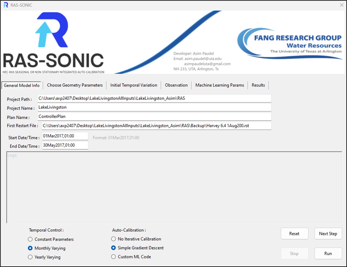
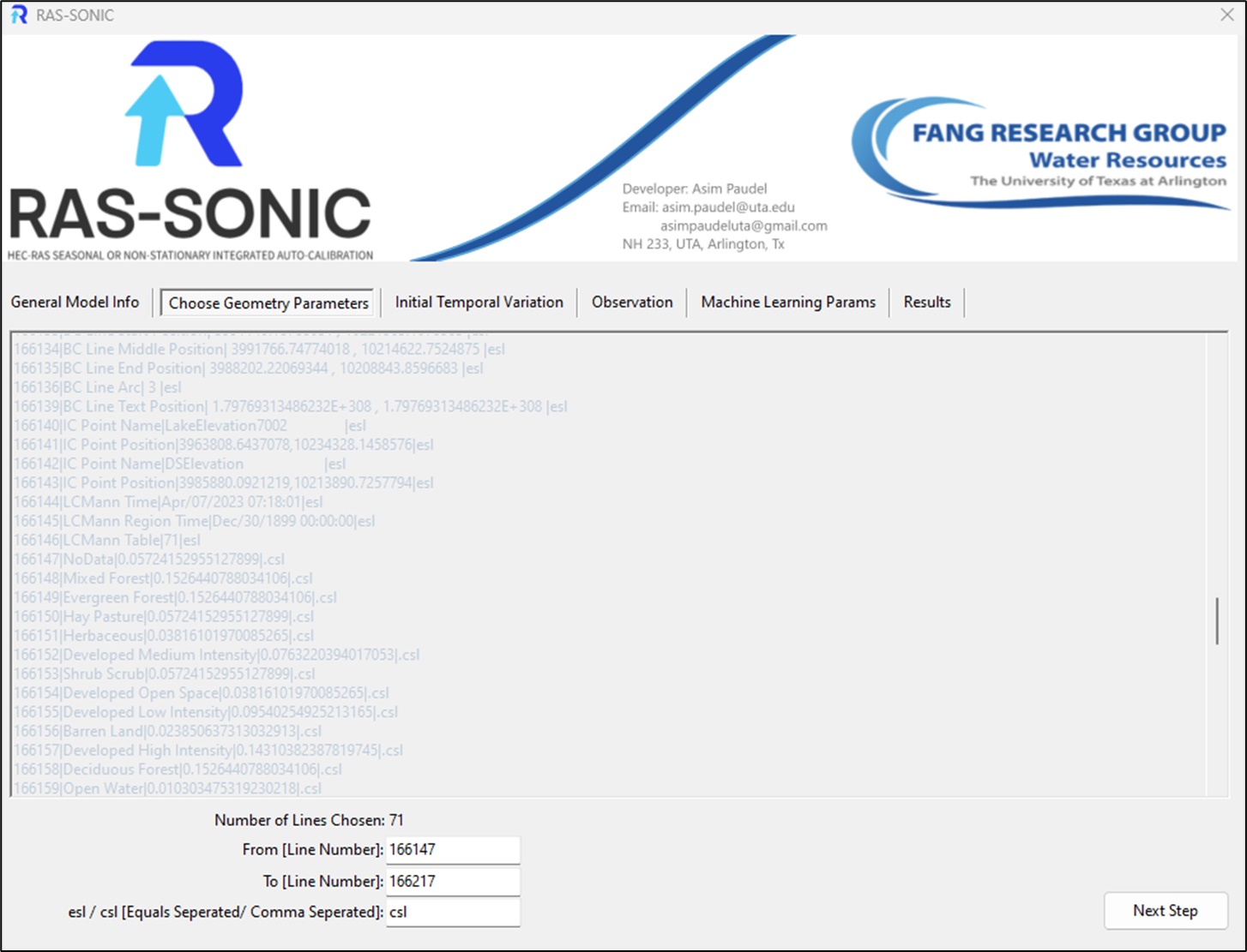
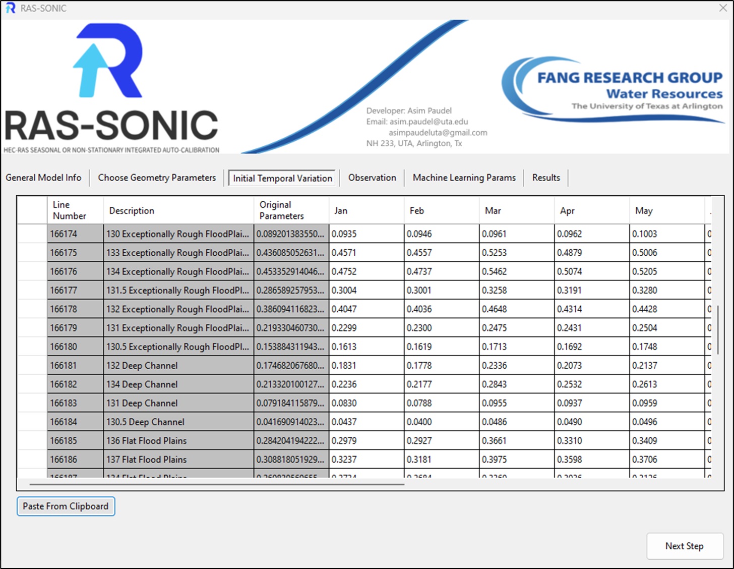
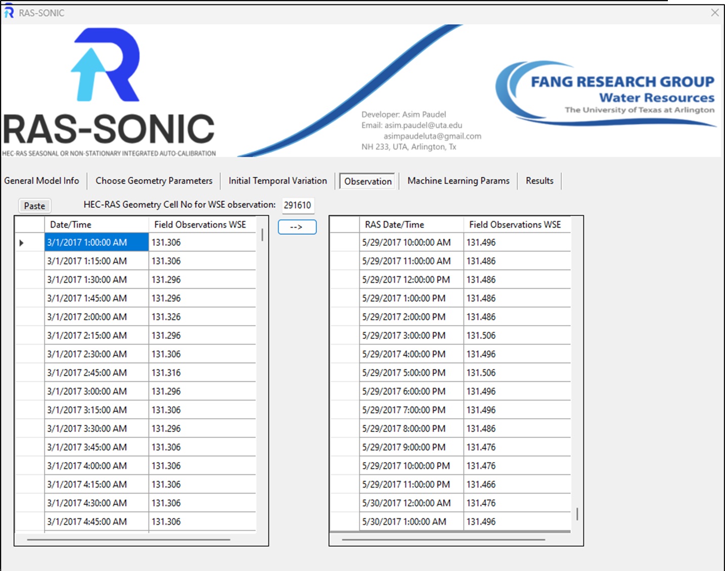
Instructions: The general input parameters are input on Tab “General Model Info” of the GUI. Upon gathering these details, the HEC-RAS software is initiated with the corresponding data loading the correct plan. Subsequently, the procedure involves the extraction of data pertinent to the plan associations, specifically focusing on geometry, unsteady flow, and plan output files. Furthermore, paths to certain output files, which will be required at later stages of analysis, are assigned. It warrants mention that the program will not enable the “RUN” button if all the required parameter in any required tabs remain unfilled or are erroneous. On tab “Choose Geometry Parameters” the program reads the geometry file and displays a list of values separated by pipe symbol “|” as well as if they are “,” comma separated values or “=” equals to separated values in the geometry file. The line numbers of parameters of interest are the required inputs. The chosen parameters in the previous step will show up on the “Initial Temporal Variation” tab. The initial values for these parameters are entered here. The next tab “Observation” requires that you input your field observation WSE for the program to compare its model run with. This will require selecting a cell number from HEC-RAS 2D geometry and pasting the observation values from a tabular data source like excel, csv or tab-delimited files.

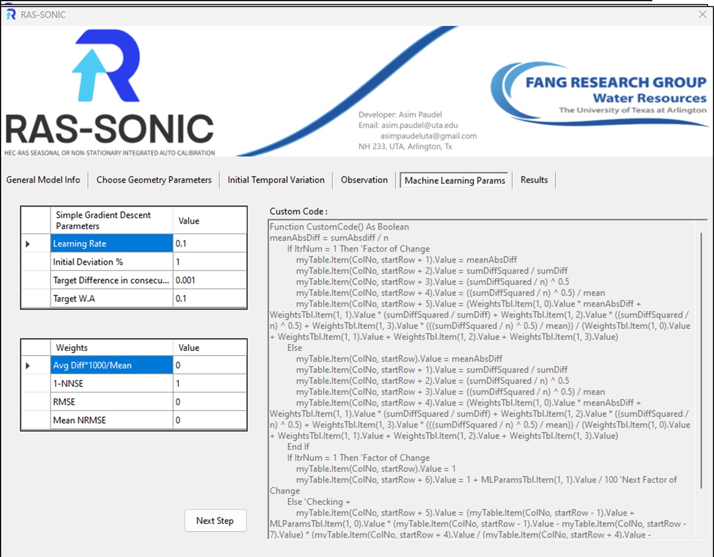
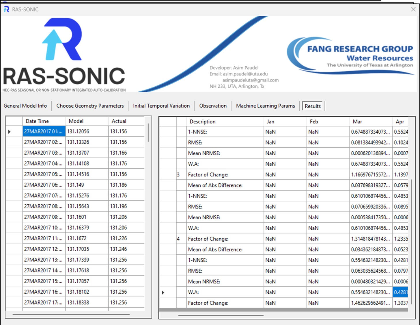
Finally, on “Machine Learning Params” tab, if simple gradient descent auto-calibration mode is selected, machine learning params will need to be input before program can be run. Various indices like mean absolute difference, NRMSE, RMSE and NNSE can be used as goodness of fit indices. They can also further be used in any weightage that the user desires. These indices of fit, along with machine learning parameters like learning rate and targets are crucial for the auto calibration algorithm. Users are also given the ability to create their own machine learning code in visual basic as a function and input it under custom code mode. This will allow users to create and share their own library of codes pertaining to their specific use cases of the software. The “Results” tab is very straightforward in that it produces the results of the temporally varied run or the calibration attempt. It gives the indices for the goodness of fit for each run and each discrete time-step. If further analysis outside RAS-SONIC is required, it also gives the last iteration WSE time-series for the entire temporal scale. The GUI has been illustrated below.

The combination of temporal control and calibration selection allows the program to be run in (3×3) distinct modes.

Temporal Variation 1.1. Constant Parameters- Constant in “Constant Parameters” refers to temporally unchanging, it may however be spatially varied. This is the default setting and is not much different compared to running the plan directly through HEC-RAS. The benefits of running it through RAS-SONIC is that the result’s goodness of fit data and WSE in the cell of interest is readily available to use upon plan completion.

1.2. Monthly Varying- This allows the user to input different parameters for different months in the year. It allows them to account for the seasonality factor in their simulation. This method is also especially useful in running long simulations without straining the computer’s storage capacity.

1.3. Yearly Varying- This allows the user to input different parameters for different years of continuous simulation. It allows them to account for the non-stationary factor in their simulation.

Learning Parameters for Auto Calibration 2.1. No Iterative Calibration- This is the base mode, which will not apply any learning algorithms.

2.2. Simple Gradient Descent: In this mode it will attempt to calibrate the parameters passed.

2.3. Custom ML Code: This is a feature wherein the users can write and share their own advanced machine learning codes. Some examples would be advanced neural networks or limits in how far learning can push any individual parameter, etc.

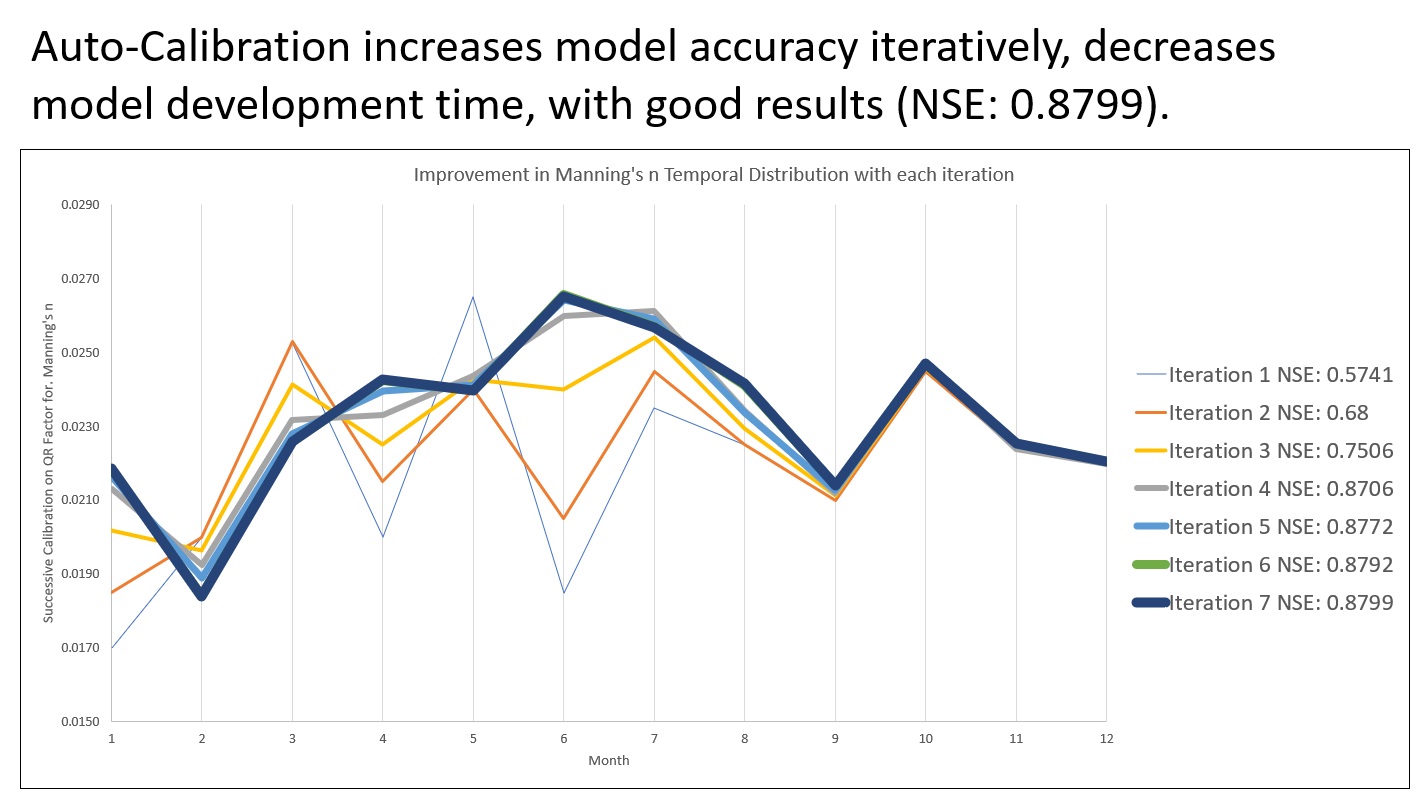
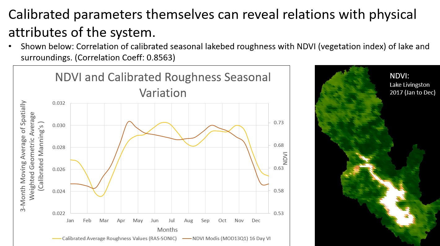
The modes can be mixed and matched for various combinations. An example is Monthly-Varying with Simple Gradient Descent. This will allow users to understand the seasonal variation in their input physical parameters.

Cite:
Asim Paudel, Dongfeng Li, & Zheng N. Fang. (2024). RAS2SONIC: HEC-RAS Seasonal or Non-stationary Integrated Calibration Package for 2D with Machine Learning Features. Environmental Modelling and Software, In Review.

Download RAS-SONIC

By downloading the software you understand that this is an experimental project, we do not in any form guarantee the efficacy of the software. Make thorough backup of your project before using it through RAS-SONIC. Reverse engineering and modification of internal code is not allowed. Internal code is proprietary and confidential. Academic use is allowed. All other rights reserved.
© November 2023| Asim Paudel.